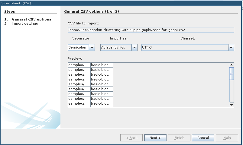
General CSV options: Adjacency list
New malware is often attributed to old malware via code similarity, or as some vendors call it malware DNA or malware genome analysis.
Here I’ll describe a simple PoC of such a “DnA GeNoMe mAlWaRe AtTrIbUtIoN EnGiNe”.
It uses two features
to cluster malware together based on their code similarity.
First, Radare2 is used via r2pipe to extract the strings of the binary via:
r2 = r2pipe.open(path, flags=['-2'])
r2.cmd('aaaa')

strings_json = r2.cmdj('izj')

strings = []

for s in strings_json:
        # FIXME: we "loose" the encoding in s['type'] here
        # so a utf-8 strings will be treated the same as the same string but in ascii
        s = base64.b64decode(s['string'])
        strings.append( [hashlib.sha256(s).hexdigest(), s.decode('utf-8')] )
Next, the basic blocks are extracted via:
results = r2.cmd('pdbj @@ *').split('\n')
results.remove('')

temp = set()

for r in results:
        temp.add(r)
temp = list(temp)

bb = []

for t in temp:
        tbb = json.loads(t)
        offset = tbb[0]['offset']
        code = b''
        for b in tbb:
                code += bytes.fromhex(b['bytes'])
        bb.append(code)
After that each basic block is masked, i.e. its immediate and displacement values are overwritten (“masked”) with zeros. This ensures that basic blocks can be compared even if they are at a different memory offset in a different binary, hence would have different immediate and displacement values as these would e.g. hold memory addresses which are likely to change between binary versions. We use capstone via:
md = Cs(CS_ARCH_X86, CS_MODE_32)
md.detail = True
md.syntax = CS_OPT_SYNTAX_INTEL

def get_masked(inst):
        code = inst.bytes
        for i in range(inst.imm_offset, inst.imm_offset + inst.imm_size):
                code[i] = 0
        for i in range(inst.disp_offset, inst.disp_offset + inst.disp_size):
                code[i] = 0
        return code

masked_bb = []


for b in bb:
        masked_b = b''
        disasm_b = ''
        for i in md.disasm(b, 0):
                #print("%s\t%s\t%s\t%d\t%d" %(i.mnemonic, i.op_str, i.insn_name(), i.imm_size, i.disp_size))
                disasm_b += i.mnemonic + '\t' + i.op_str + '\n'
                force_mask = False
                for g in i.groups:
                        if i.group_name(g) in ['call', 'jump']:
                                force_mask = True
                if force_mask or i.imm_size > 1 or i.disp_size > 1:
                        masked_b += get_masked(i)
                else:
                        masked_b += i.bytes

        masked_bb.append([hashlib.sha256(masked_b).hexdigest(),disasm_b])
Last but not least we output the strings and basic blocks on tab separated lines:
for s in strings:
        print(path +'\t'+ s[0] +'\t'+ s[1])

for b in masked_bb:
        print(path +'\t'+ b[0] +'\t'+ b[1].replace('\n','; '))
That’s it. The above code is in file extract_features.py.
To allow for mass ingestion of samples and to format the output into a format that Gephi can understand we can use extract_all.sh:
#!/bin/bash

mkdir -p features
ls samples/* | while read input; do
output="$(echo "${input}" | sed 's/samples/features/g').csv"
python3 extract_features.py "${input}" > "${output}"
done

cat features/*.csv | awk -F'\t' '{print $1";basic-block-"$2}' > for_gephi.csvsamples that contains your samples into the same directory. The structure should look like:.
|-- extract_all.sh
|-- extract_features.py
`-- samples
|-- CozyDuke_f16cfb7e54a11689fc1a37145b7ff28f17a1930c74324650e9a080ac87d69ac7
|-- CozyDuke_f9987e6be134bf29458a336a76600a267e14b07a57032b6a8fc656f750e40ce5
|-- Duqu2_6e09e1a4f56ea736ff21ad5e188845615b57e1a5168f4bdaebe7ddc634912de9
|-- Duqu2_d12cd9490fd75e192ea053a05e869ed2f3f9748bf1563e6e496e7153fb4e6c98
|-- Stuxshop_32159d2a16397823bc882ddd3cd77ecdbabe0fde934e62f297b8ff4d7b89832a
|-- Stuxshop_c074aeef97ce81e8c68b7376b124546cabf40e2cd3aff1719d9daa6c3f780532
|-- TSCookie_6d2f5675630d0dae65a796ac624fb90f42f35fbe5dec2ec8f4adce5ebfaabf75
`-- TSCookie_96306202b0c4495cf93e805e9185ea6f2626650d6132a98a8f097f8c6a424a33
1 directories, 10 files./extract_all.sh. Your folder structure should now look like:.
|-- extract_all.sh
|-- extract_features.py
|-- features
| |-- CozyDuke_f16cfb7e54a11689fc1a37145b7ff28f17a1930c74324650e9a080ac87d69ac7.csv
| |-- CozyDuke_f9987e6be134bf29458a336a76600a267e14b07a57032b6a8fc656f750e40ce5.csv
| |-- Duqu2_6e09e1a4f56ea736ff21ad5e188845615b57e1a5168f4bdaebe7ddc634912de9.csv
| |-- Duqu2_d12cd9490fd75e192ea053a05e869ed2f3f9748bf1563e6e496e7153fb4e6c98.csv
| |-- Stuxshop_32159d2a16397823bc882ddd3cd77ecdbabe0fde934e62f297b8ff4d7b89832a.csv
| |-- Stuxshop_c074aeef97ce81e8c68b7376b124546cabf40e2cd3aff1719d9daa6c3f780532.csv
| |-- TSCookie_6d2f5675630d0dae65a796ac624fb90f42f35fbe5dec2ec8f4adce5ebfaabf75.csv
| `-- TSCookie_96306202b0c4495cf93e805e9185ea6f2626650d6132a98a8f097f8c6a424a33.csv
|-- for_gephi.csv
`-- samples
|-- CozyDuke_f16cfb7e54a11689fc1a37145b7ff28f17a1930c74324650e9a080ac87d69ac7
|-- CozyDuke_f9987e6be134bf29458a336a76600a267e14b07a57032b6a8fc656f750e40ce5
|-- Duqu2_6e09e1a4f56ea736ff21ad5e188845615b57e1a5168f4bdaebe7ddc634912de9
|-- Duqu2_d12cd9490fd75e192ea053a05e869ed2f3f9748bf1563e6e496e7153fb4e6c98
|-- Stuxshop_32159d2a16397823bc882ddd3cd77ecdbabe0fde934e62f297b8ff4d7b89832a
|-- Stuxshop_c074aeef97ce81e8c68b7376b124546cabf40e2cd3aff1719d9daa6c3f780532
|-- TSCookie_6d2f5675630d0dae65a796ac624fb90f42f35fbe5dec2ec8f4adce5ebfaabf75
`-- TSCookie_96306202b0c4495cf93e805e9185ea6f2626650d6132a98a8f097f8c6a424a33
2 directories, 19 filesfor_gephi.csv in Gephi (File -> Import spreadsheet…) and import as adjacency list.General CSV options: Adjacency list
Import settings: Just click “Finish”
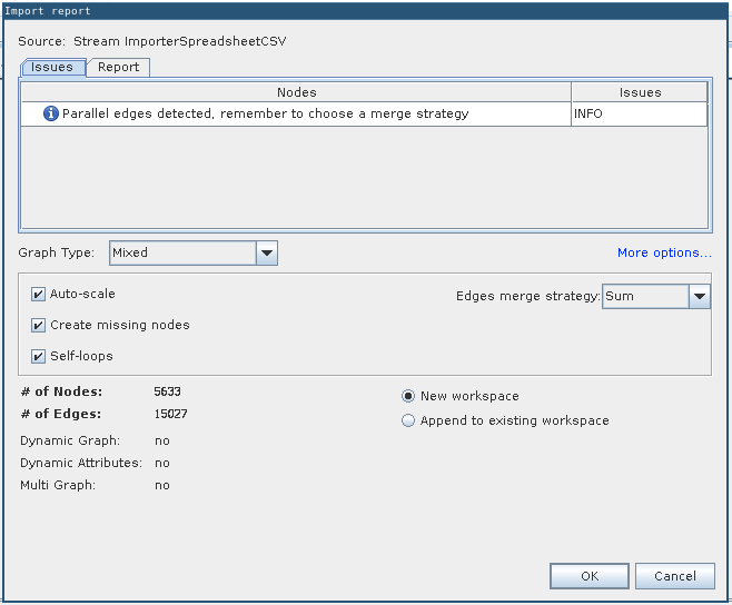
Import report with no errors
Next goto “Data Laboratory”, select all nodes, right-click and select “Edit node”.
In the Properties set Size to 1.0 and color to Light Gray.
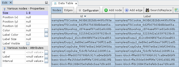
Node Properties for the basic blocks
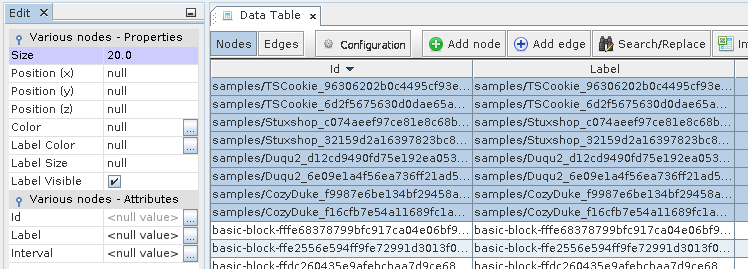
Node Properties Size for the samples
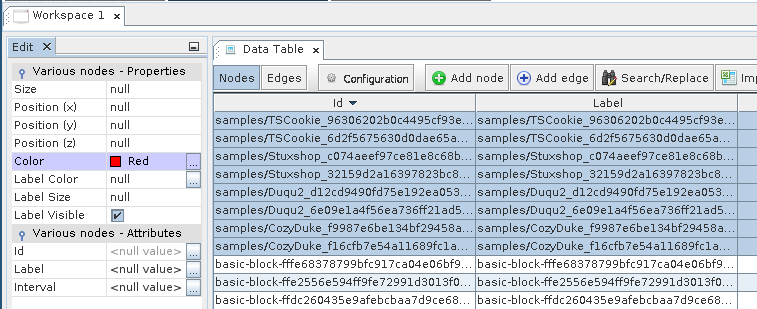
Node Properties Color for the samples
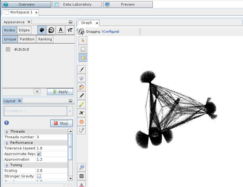
ForceAltlas 2 Layout
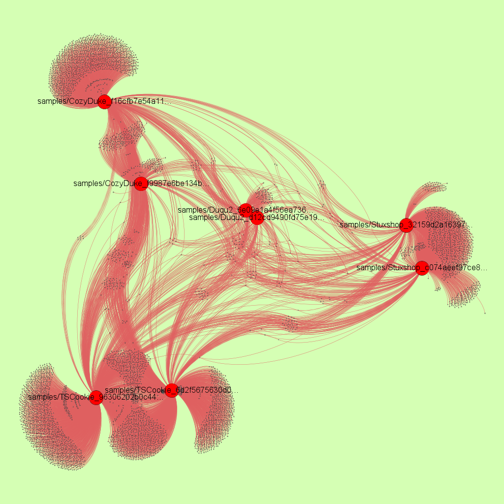
6 samples clustered with r2pipe, capstone and Gephi
Update 1: 11. Spend more time with colors and applying the “Yifan Hu” Layout followed by a short burst of “ForceAtlas 2” to prevent overlaps you get really cool looking clustering graphics:
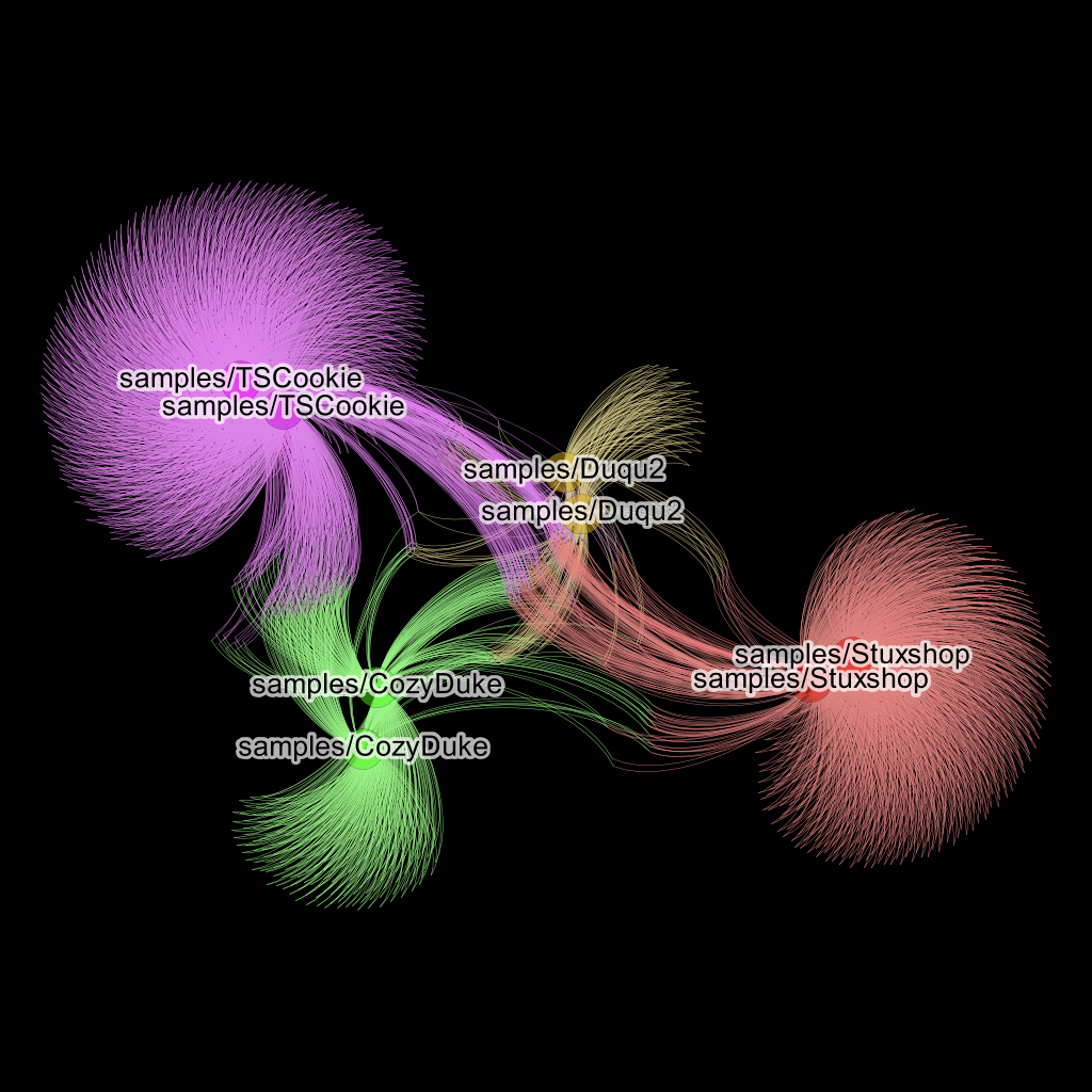
Same graphic as before but made cooler by color and black background.
As can be seen from the resulting image each two related malware samples are clustered together, i.e. pulled closer together in the force directed graph by their basic block and string edges.
Obviously, real attribution takes way more effort than this simple PoC. However, the code and string similarity matching is accurate. So if a masked basic block is in two samples, it means that these two samples share code - or at least that basic block. Here it is important that the shared code is meaningful, e.g., a lot of binaries share library code. Trivial basic block that have only few instructions obviously also don’t indicate meaningful code sharing, however, if you can find several basic blocks from key functions shared between samples it is very likely that they are related.
While I used Gephi to cluster via a force directed graph you could also simply calculate the amount of shared basic blocks or use other metrics to bin different binaries together based on feature similarity.
I hope this simple PoC can get someone started with their shared code and code similarity analysis. If you do something cool based on this give me a shout - I’d like to see it.